Variational Auto-Encoders and the Reparameterization Trick
Having spent the last half a year or so working on variational inference for my thesis, I don’t consider myself an expert at it, but I’m a whole lot more knowledgable than I was two years ago when I got the idea into my head that the only way machine learning could result in something that is actually capable of reasoning in a “smart” way was by using a Bayesian approach. It made perfect sense to me, but I was lacking the mathematical and theoretical foundations to utilize this idea. So now that I’ve spent so many hours dealing with the subject, I wanted to write some kind of a tutorial that would make my former self understand the beauty of the Variational Auto-Encoder — and maybe it would also be useful for somebody else in the same position.
Deterministic Auto-Encoders
I won’t go into any detail on neural nets and their variants, as much has been written by folks smarter than me - I recommend Karpathy’s blog as a start point. The multi-layer perceptron and the auto-encoder were pretty much my very first exposure to machine learning, some six years ago, and I was fascinated by them right off the bat. What was not immediately clear to me, however, was the fact that different-dimensional real spaces do not necessarily represent a “smaller” or “bigger” place than each other. Anything infinite is always confusing to me (and most humans probably) and it took a step back from intuitive reasoning to looking at just the math in order for me to get to grip with the fact that you can (within reason — it gets complicated when you’re talking about countable and uncountable infinities) find a bijective mapping from just about any inifinite set to another. So what is an auto-encoder really doing? Well, if you use weight regularization and tricks like that, you can certainly ensure some compression in the bottleneck layer, but it’s rather hit or miss getting it to work.
Variational Bayes
A few years ago a clever model called the Variational Auto-Encoder (or VAE) was invented. As is so often the case, the theoretical breakthrough was made by several teams in parallel, more or less at the same time. Although the VAE shares two thirds of its name as well as most of its structure superficially with the auto-encoder, the underlying idea is rather different and more grounded in mathematical theory. Taking a probabilistic approach, one assumes that the data being examined are samples from a random variable called the observation x. This random variable is not fully independent, but rather depends on some unobservable latent factors z. It would be lovely if it were simply possible to determine the latent factors z from looking at observations, but this is in all but the most trivial cases intractable. Instead one assumes that the distributions in question are parametrizable and attempts to learn them using neural networks.
In the simplest case all distributions in question are Gaussians, which can be described by their sufficient statistics mean and (co)variance. This assumption makes many things easier, so I shall stick with it throughout the rest of this post, but in principle there is nothing stopping one from using any distribution that can be parameterized and is differentiable — also there is no reason why x and z must be of the same class of distribution.
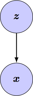
The first thing to learn is the generative or forward model, which is to say the conditional dependencies of the real underlying process that generate samples of x based on a given latent z — or at least a good approximation to it. Given known pairs of latents and observations, it’s easy to train a neural network using back-propagation to predict p(x|z). Expressed as a probabilistic graphical model (PGM) the generative network looks something like this: